Local Senstivity Analysis • MEMC

The objective of this example is demonstrate how to use memc_sensfun to conduct a local sensitivity analysis and visualize the results to demonstrate package capabilities.

The memc_sensfun function is a wrapper for sensFun from the FME package, designed to help memc users easily perform a local sensitivity analysis on any memc parameter or initial condition. The official FME provides more details, but in short, memc_sensfun runs a memc configuration multiple times: first as a reference run, then as a series of perturbation runs—one for each parameter of interest. During each perturbation run, a single parameter is changed slightly while others remain constant. The output of memc_sensfun includes the numerical approximations of partial derivatives, representing the sensitivity of the model output to each perturbed parameter.

Start by loading the packages used in the demonstration.

library(MEMC) 


library(ggplot2)
theme_set(theme_bw())

Select the memc parameters or initial conditions to include in the local sensitivity analysis. Any of the parameters included in memc_params or memc_initial_state may be considered. In this example we will consider how the memc MEND configuration is sensitive to $V_d$ and $K_d$ , the maximum and half saturation rates of DOM decomposition.

Create a vector of the parameter values of interest, the ones we would like to consider in the local sensitivity analysis and set equal to the the parameter values used by the memc_config that will be used to run memc_sensfun.

params_to_perturb <- c("V_d" =  3, "K_d" = 0.25)

Run the local sensitivity analysis for a memc configuration. The config may be any of the default configuraitons listed in memc_all_configs or one created by a user via memc_configure.

out1 <- memc_sensfun(config = MEND_config,     
                     t = 0:100, 
                     x = params_to_perturb)

The returned data frame includes details about the simulation, such as its name, time, and pool. The value column contains the partial derivative of the simulation output with respect to the perturbed parameter, which is specified in the parameter column.

head(out1)
#>      name  time variable parameter        value
#>    <char> <num>   <char>    <fctr>        <num>
#> 1:   MEND     0      POM       V_d  0.000000000
#> 2:   MEND     1      POM       V_d  0.048743867
#> 3:   MEND     2      POM       V_d  0.033570845
#> 4:   MEND     3      POM       V_d  0.015965606
#> 5:   MEND     4      POM       V_d  0.004513539
#> 6:   MEND     5      POM       V_d -0.001963303

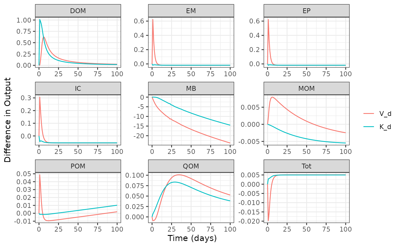
Quickly plot the results to compare how parameter perturbations affect model output across all pools throughout the simulation.

plot(out1)

Now let’s apply memc_sensfun to an other model configuration so that we may compare the results.

out2 <- memc_sensfun(config = CORPSE_config,     
                     t = 0:100, 
                     x = params_to_perturb)
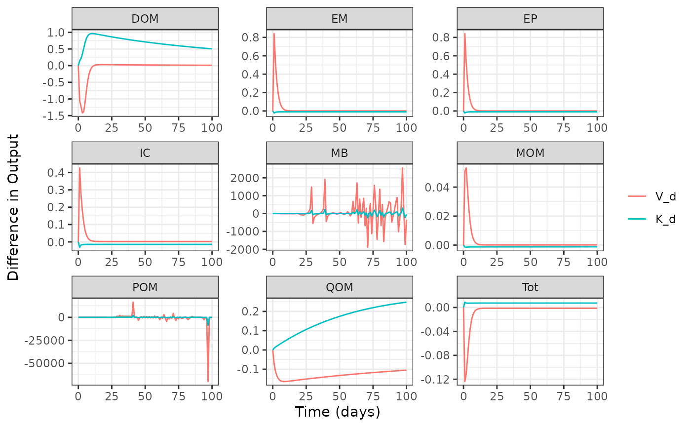
plot(out2)

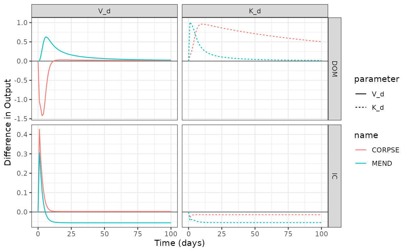
Figures 1 and 2 are quite different from one another, let’s focus on the DOM and IC pools in a side by side comparison. But first recall what is different between these two configurations. By taking a look at their configuration tables. It appears that these models differ in how the represent DOM uptake and POM decomposition.

rbind(MEND_config$table, 
      CORPSE_config$table)
#>    model DOMuptake POMdecomp MBdecay
#> 1   MEND        MM        MM      LM
#> 2 CORPSE       RMM        LM      LM

# Save results for the two carbon pools are we are interested in. 
out1_to_compare <- out1[out1$variable %in% c("DOM", "IC"), ]
out2_to_compare <- out2[out2$variable %in% c("DOM", "IC"), ]

# Combine into a single data frame for plotting 
to_plot <- rbind(out1_to_compare, out2_to_compare)


# Plot the results 
ggplot(data = to_plot) + 
  geom_hline(yintercept = 0, alpha = 0.5) + 
  geom_line(aes(time, value, color = name, linetype = parameter)) + 
  facet_grid(variable ~ parameter, scales = "free") + 
  labs(y  = "Difference in Output", x = "Time (days)")

The figure above demonstrate how MEND and CORPSE ROM and IC pools respond differently to parameter perturbations.